Preliminaries #1: Diffusion Models
Overview
This blog aims to provide an intuitive introduction to Diffusion Models. For further in-depth reading, several highly recommended blogs are available:
- For beginners:
- Understanding Diffusion Models: A Unified Perspective by Calvin Luo
- For more details:
- What are Diffusion Models? by Lilian Weng
- Generative Modeling by Estimating Gradients of the Data Distribution by Yang Song
Given observed samples $x$ from a distribution of interest, the goal of a generative model is to learn to model its true data distribution $p(x)$. Once learned, we can generate new samples from our approximate model at will. Furthermore, under some formulations, we are able to use the learned model to evaluate the likelihood of observed or sampled data as well.
Background
VAE & ELBO
Before introducing Diffusion Model, let’s just revise the Variational AutoEncoder (VAE) and Evidence Lower Bound (ELBO).
Variational Autoencoder introduced a latent variable $z$ to learn the underlying latent structure that describes our observed data $x$. For training a VAE, we learn an intermediate bottlenecking distribution $q_\phi(z|x)$ that can be treated as an encoder; it transforms inputs into a distribution over possible latents. Simultaneously, we learn a deterministic function $p_\theta(x|z)$ to convert a given latent vector $z$ into an observation $x$, which can be interpreted as a decoder.
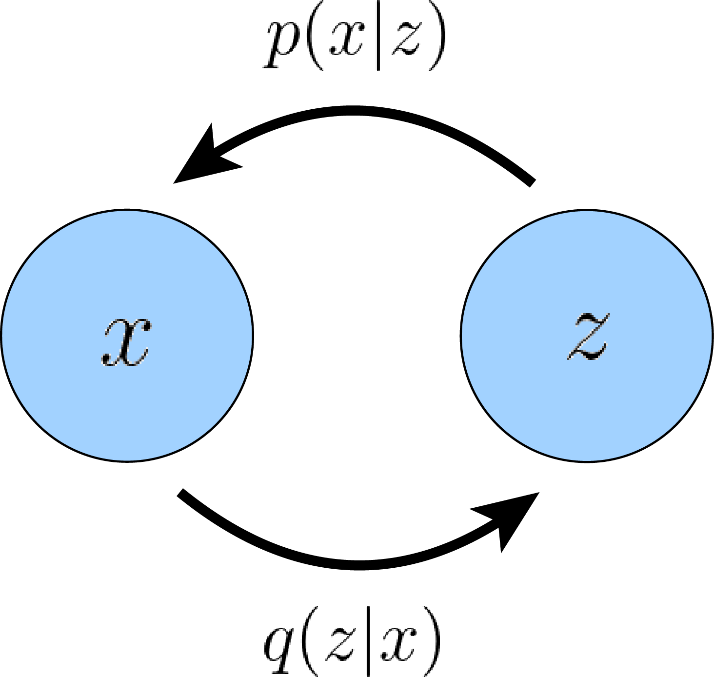
A latent encoder and decoder are learned jointly through the reparameterization trick.
Mathematically, we can imagine the latent variables and the data we observe as modeled by a joint distribution $p(x, z)$. Likelihood-based generative modeling, like VAE, learns a model to maximize the likelihood $p(x)$ of all observed $x$. There are two ways we can manipulate this joint distribution to recover the likelihood of purely our observed data $p(x)$ ; we can explicitly marginalize out the latent variable $z$:
or, we could also appeal to the chain rule of probability:
Using these two equations, we can derive a term called the Evidence Lower Bound (ELBO).
Evidence Lower Bound (ELBO), which as its name suggests, is a lower bound of the evidence. In this case, the evidence is quantified as the log likelihood of the observed data, denoted as $\log p(x)$.
Let’s derive ELBO using the chain rule marginalization method, as in Equation 2:
Derive ELBO using the integration marginalization and Jensen's inequality (optional)
There's an alternative method to derive ELBO from evidence, commonly found in blogs introducing Diffusion Models. However, I don't personally recommend this approach as it fails to provide sufficient intuition as to why we opt for ELBO to optimize generative models.Jensen’s inequality states that for any concave function $f(x)$, if $X$ is a random variable, then:
Let’s start from Equation 1, we can derive ELBO:
In this derivation, we directly arrive at our lower bound by applying Jensen’s Inequality. However, this does not supply us much useful information about what is actually going on underneath the hood; crucially, this proof gives no intuition on exactly why the ELBO is actually a lower bound of the evidence, as Jensen’s Inequality handwaves it away. Furthermore, simply knowing that the ELBO is truly a lower bound of the data does not really tell us why we want to maximize it as an objective.
We can rewrite ELBO into a form of VAE objective:
- reconstruction term measures the reconstruction likelihood of the decoder from our variational distribution; this ensures that the learned distribution is modeling effective latents that the original data can be regenerated from.
- prior matching term measures how similar the learned variational distribution is to a prior belief held over latent variables. Minimizing this term encourages the encoder to actually learn a distribution rather than collapse into a Dirac delta function.
Variational is the term used for variational inference, a technique that approximates complex probability distributions using simpler ones. It finds the distribution in a specific class that is closest to the true posterior distribution. In VAE, it refers to the fact that we optimize for the best $q_\phi(z|x)$ amongst a family of potential posterior distributions parameterized by $\phi$.
After training a VAE, generating new data can be performed by sampling directly from the latent space and then running it through the learned decoder.
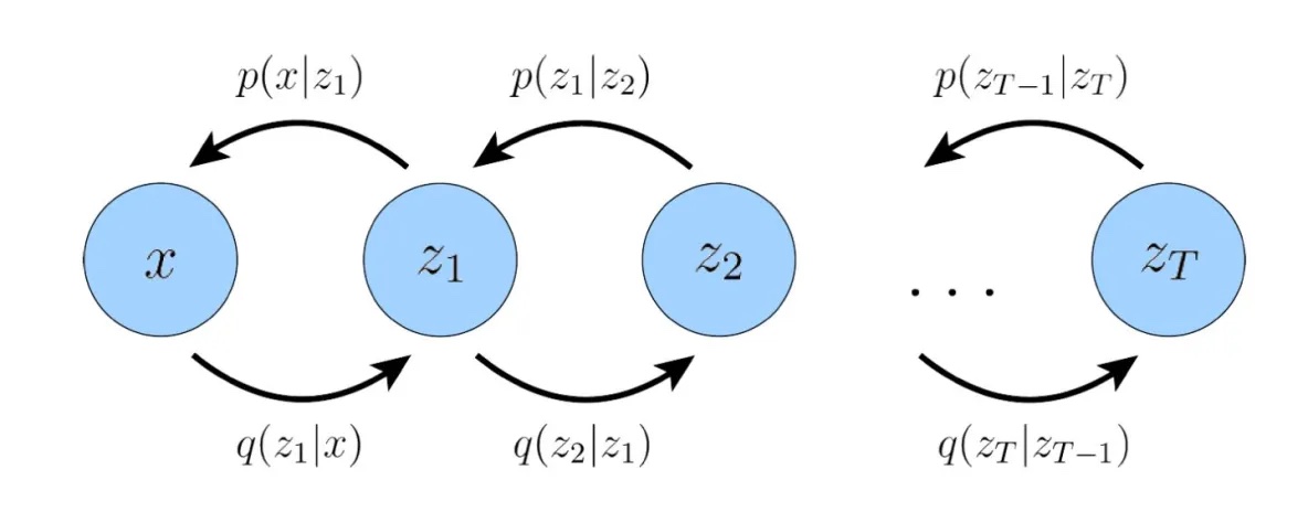
HVAE
Hierarchical Variational Autoencoder (HVAE) is a generalization of a VAE that extends to multiple hierarchies over latent variables. Under this formulation, latent variables themselves are interpreted as generated from other higher-level, more abstract latents.